LibFile: isosurface.scad
Metaballs (also known as "blobby objects"), are bounded and closed organic surfaces that smoothly blend together. Metaballs are a specific kind of isosurface.
An isosurface, or implicit surface, is a three-dimensional surface representing all points of a constant value (e.g. pressure, temperature, electric potential, density) in a 3D volume. It's the 3D version of a 2D contour; in fact, any 2D cross-section of an isosurface is a 2D contour.
For computer-aided design, isosurfaces of abstract functions can generate complex curved surfaces and organic shapes. For example, spherical metaballs can be formulated using a set of point centers that define the metaballs locations. For metaballs, a function is defined for all points in a 3D volume based on the distance from any point to the centers of each metaball. The combined contributions from all the metaballs results in a function that varies in a complicated way throughout the volume. When two metaballs are far apart, they appear simply as spheres, but when they are close together they enlarge, reach toward each other, and meld together in a smooth fashion. The resulting metaball model appears as smoothly blended blobby shapes. The implementation below provides metaballs of a variety of types including spheres, cuboids, and cylinders (cones), with optional parameters to adjust the influence of one metaball on others, and the cutoff distance where the metaball's influence stops.
In general, an isosurface can be defined using any function of three variables x, y, z.
The isosurface of a function f(x,y,z) is the set of points where f(x,y,z)=c for some constant
value c. Such a function is also known as an "implied surface" because the function implies a
surface of constant value within a volume of space. The constant c is referred to as the "isovalue".
Changing the isovalue changes the position of the isosurface, depending on how the function is
defined. Because metaballs are isosurfaces, they also have an isovalue. The isovalue is also known
as the "threshold".
Some isosurface functions are unbounded, extending infinitely in all directions. A familiar example may be a gryoid, which is often used as a volume infill pattern in fused filament fabrication. The gyroid isosurface is unbounded and periodic in all three dimensions.
This file provides modules and functions to create a VNF using metaballs, or from general isosurfaces.
To use, add the following lines to the beginning of your file:
include <BOSL2/std.scad>
include <BOSL2/isosurface.scad>
File Contents
metaballs()– Creates a group of 3D metaballs (smoothly connected blobs). [Geom] [VNF]isosurface()– Creates a 3D isosurface (a 3D contour) from a function or array of values. [Geom] [VNF]
Function/Module: metaballs()
Synopsis: Creates a group of 3D metaballs (smoothly connected blobs). [Geom] [VNF]
Topics: Metaballs, Isosurfaces, VNF Generators
See Also: isosurface()
Usage: As a module
- metaballs(spec, voxel_size, bounding_box, [isovalue=], [closed=], [convexity=], [show_stats=], ...) [ATTACHMENTS];
Usage: As a function
- vnf = metaballs(spec, voxel_size, bounding_box, [isovalue=], [closed=], [convexity=], [show_stats=]);
Description:
Metaballs, also known as "blobby objects", can produce smoothly varying blobs and organic forms. You create metaballs by placing metaball objects at different locations. These objects have a basic size and shape when placed in isolation, but if another metaball object is nearby, the two objects interact, growing larger and melding together. The closer the objects are, the more they blend and meld.
The simplest metaball specification is a 1D list of alternating transformation matrices and
metaball functions: [trans0, func0, trans1, func1, ... ]. Each transformation matrix
you supply can be constructed using the usual transformation commands such as up(),
right(), back(), move(), scale(), rot() and so on. You can multiply
the transformations together, similar to how the transformations can be applied
to regular objects in OpenSCAD. For example, to transform an object in regular OpenSCAD you
might write up(5) xrot(25) zrot(45) scale(4). You would provide that transformation
as the transformation matrix up(5) * xrot(25) * zrot(45) * scale(4). You can use
scaling to produce an ellipsoid from a sphere, and you can even use skew() if desired.
When no transformation is needed, give IDENT as the transformation.
The metaballs are evaluated over a bounding box defined by its minimum and maximum corners,
[[xmin,ymin,zmin],[xmax,ymax,zmax]]. The contributions from all metaballs, even those outside
the bounds, are evaluated over the bounding box. This bounding box is divided into voxels of the
specified voxel_size. Smaller voxels produce a finer, smoother result at the expense of
execution time. If the voxel size doesn't exactly divide your specified bounding box, then
the bounding box is enlarged to contain whole voxels, and centered on your requested box. If
the bounding box clips a metaball and closed=true (the default), the object is closed at the
intersection surface. Setting closed=false causes the VNF to end at the bounding box,
resulting in a non-manifold shape with holes, exposing the inside of the object.
For metaballs with flat surfaces (the ends of mb_cyl(), and mb_cuboid() with squareness=1),
avoid letting any side of the bounding box coincide with one of these flat surfaces, otherwise
unpredictable triangulation around the edge may result.
You can create metaballs in a variety of standard shapes using the predefined functions
listed below. If you wish, you can also create custom metaball shapes using your own functions
(see Example 19). For all of the built-in metaballs, three parameters are availableto control the
interaction of the metaballs with each other: cutoff, influence, and negative.
The cutoff parameter specifies the distance beyond which the metaball has no interaction
with other balls. When you apply cutoff, a smooth suppression factor begins
decreasing the interaction strength at half the cutoff distance and reduces the interaction to
zero at the cutoff. Note that the smooth decrease may cause the interaction to become negligible
closer than the actual cutoff distance, depending on the voxel size and influence of the
ball. Also, depending on the value of influence, a cutoff that ends in the middle of
another ball can result in strange shapes, as shown in Example 16, with the metaball
interacting on one side of the boundary and not interacting on the other side. If you scale
a ball, the cutoff value is also scaled. The exact way that cutoff is defined
geometrically varies for different ball types; see below for details.
The influence parameter adjusts the strength of the interaction that metaball objects have with
each other. If you increase influence of one metaball from its default of 1, then that metaball
interacts with others at a longer range, and surrounding balls grow bigger. The metaball with larger
influence can also grow bigger because it couples more strongly with other nearby balls, but it
can also remain nearly unchanged while influencing others when isovalue is greater than 1.
Decreasing influence has the reverse effect. Small changes in influence can have a large
effect; for example, setting influence=2 dramatically increases the interactions at longer
distances, and you may want to set the cutoff argument to limit the range influence.
The negative parameter, if set to true, creates a negative metaball, which can result in
hollows or dents in other metaballs, or swallow other metaballs almost entirely.
Negative metaballs are always below the isovalue, so they are never directly visible;
only their effects are visible. See Examples 15 and 16.
The isovalue parameter in metaballs() defaults to 1. If you increase it, then all the objects
in your model shrink, causing some melded objects to separate. If you decrease it, each metaball
grows and melds more with others. Be aware that changing the isovalue affects all the metaballs
and changes the entire model, possibly dramatically.
For complicated metaball assemblies you may wish to repeat a structure in different locations or
otherwise transformed. Nested metaball specifications are supported:
Instead of specifying a transform and function, you specify a transform and then another metaball
specification. For example, you could set finger=[t0,f0,t1,f1,t2,f2] and then set
hand=[u0,finger,u1,finger,...] and then invoke metaballs() with [s0, hand].
In effect, any metaball specification array can be treated as a single metaball in another specification array.
This is a powerful technique that lets you make groups of metaballs that you can use as individual
metaballs in other groups, and can make your code compact and simpler to understand. See Example 21.
Built-in metaball functions
Several metaballs are defined for you to use in your models.
All of the built-in metaballs take positional and named parameters that specify the size of the
metaball (such as height or radius). The size arguments are the same as those for the regular objects
of the same type (e.g. a sphere accepts both r for radius and the named parameter d= for
diameter). The size parameters always specify the size of the metaball in isolation with
isovalue=1. The metaballs can grow much bigger than their specified sizes when they interact
with each other. Changing isovalue also changes the sizes of metaballs. They grow bigger than their
specified sizes, even in isolation, if isovalue < 1 and smaller than their specified sizes if
isovalue > 1.
All of the built-in functions accept these named arguments, which are not repeated in the list below:
cutoff— positive value giving the distance beyond which the metaball does not interact with other balls. Cutoff is measured from the object's center unless otherwise noted below. Default: INFinfluence— a positive number specifying the strength of interaction this ball has with other balls. Default: 1negative— when true, creates a negative metaball. Default: false
The built-in metaball functions are listed below. As usual, arguments without a trailing = can be used positionally; arguments with a trailing = must be used as named arguments.
The examples below illustrates each type of metaball interacting with another of the same type.
mb_sphere(r|d=)— spherical metaball, with radius r or diameter d. You can create an ellipsoid usingscale()as the last transformation entry of the metaballspecarray.mb_cuboid(size, [squareness=])— cuboid metaball with rounded edges and corners. The corner sharpness is controlled by thesquarenessparameter ranging from 0 (spherical) to 1 (cubical), and defaults to 0.5. Thesizespecifies the width of the cuboid shape between the face centers;sizemay be a scalar or a vector, as incuboid(). Except whensquareness=1, the faces are always a little bit curved.mb_cyl(h|l|height|length, [r|d=], [r1=|d1=], [r2=|d2=], [rounding=])— vertical cylinder or cone metaball with the same dimenional arguments ascyl(). At least one of the radius or diameter arguments is required. Theroundingargument defaults to 0 (sharp edge) if not specified. Only one rounding value is allowed: the rounding is the same at both ends. For a fully rounded cylindrical shape, consider usingmb_capsule()ormb_disk(), which are less flexible but have faster execution times. For this metaball, the cutoff is measured from surface of the cone with the specified dimensions.mb_disk(h|l|height|length, r|d=)— rounded disk with flat ends. The diameter specifies the total diameter of the shape including the rounded sides, and must be greater than its height.mb_capsule(h|l|height|length, r|d=)— cylinder of radiusror diameterdwith hemispherical caps. The height or length specifies the total height including the rounded ends.mb_connector(p1, p2, r|d=)— a connecting rod of radiusror diameterdwith hemispherical caps (likemb_capsule()), but specified to connect pointp1to pointp2(wherep1andp2must be different 3D coordinates). The specified points are at the centers of the two capping hemispheres. You may want to setinfluencequite low; the connectors themselves are still influenced by other metaballs, but it may be undesirable to have them influence others, or each other. If two connectors are connected, the joint may appear swollen unlessinfluenceis reduced.mb_torus([r_maj|d_maj=], [r_min|d_min=], [or=|od=], [ir=|id=])— torus metaball oriented perpendicular to the z axis. You can specify the torus dimensions using the same arguments astorus(); that is, major radius (or diameter) withr_majord_maj, and minor radius and diameter usingr_minord_min. Alternatively you can give the inner radius or diameter withiroridand the outer radius or diameter withororod. Both major and minor radius/diameter must be specified regardless of how they are named. *mb_octahedron(r|d=])— octahedral metaball with sharp edges and corners. Therparameter specifies the distance from center to tip, whiled=is the distance between two opposite tips.
Metaball functions and user defined functions
Each metaball is defined as a function of a 3-vector that gives the value of the metaball function
for that point in space. As is common in metaball implementations, we define the built-in metaballs using an
inverse relationship where the metaball functions fall off as 1/d, where d is distance from the
metaball center. The spherical metaball therefore has a simple basic definition as f(v) = 1/norm(v).
With this framework, f(v) >= c defines a bounded object. Increasing the isovalue shrinks the
object, and decreasing the isovalue grows the object.
To adjust interaction strength, the influence parameter applies an exponent, so if influence=a
then the decay becomes \frac{1}{d^{\frac 1 a}}. This means, for example, that if you set influence to
0.5 you get a \frac{1}{d^2} falloff. Changing this exponent changes how the balls interact.
You can pass a custom function as a function literal that takes a single argument (a 3-vector) and returns a single numerical value. The returned value should define a function where in isovalue range [c,INF] defines a bounded object. See Example 19 for a demonstration of creating a custom metaball function.
Voxel size and bounding box
The voxel_size and bounding_box parameters affect the run time, which can be long.
A voxel size of 1 with a bounding box volume of 200×200×200 may be slow because it requires the
calculation and storage of 8,000,000 function values, and more processing and memory to generate
the triangulated mesh. On the other hand, a voxel size of 5 over a 100×100×100 bounding box
requires only 8,000 function values and a modest computation time. A good rule is to keep the
number of voxels below 10,000 for preview, and adjust the voxel size smaller for final
rendering. A bounding box that is larger than your isosurface wastes time computing function
values that are not needed. If the metaballs fit completely within the bounding box, you can
call pointlist_bounds() on vnf[0] returned from the metaballs() function to get an
idea of a the optimal bounding box to use. You may be able to decrease run time, or keep the
same run time but increase the resolution. You can also set the parameter show_stats=true to
get the bounds of the voxels containing the generated surfaces.
The point list in the returned VNF structure contains many duplicated points. This is not a
problem for rendering the shape, but if you want to eliminate these, you can pass
the structure to vnf_merge_points(). Additionally, flat surfaces (often
resulting from clipping by the bounding box) are triangulated at the voxel size
resolution, and these can be unified into a single face by passing the vnf
structure to vnf_unify_faces(). These steps can be computationally expensive
and are not normally necessary.
Arguments:
| By Position | What it does |
|---|---|
spec |
Metaball specification in the form [trans0, spec0, trans1, spec1, ...], with alternating transformation matrices and metaball specs, where spec0, spec1, etc. can be a metaball function or another metaball specification. See above for more details, and see Example 21 for a demonstration. |
voxel_size |
scalar size of the voxel cube that is used to sample the bounding box volume. |
bounding_box |
A pair of 3D points [[xmin,ymin,zmin], [xmax,ymax,zmax]], specifying the minimum and maximum box corner coordinates. The actual bounding box enlarged if necessary to make the voxels fit perfectly, and centered around your requested box. |
isovalue |
A scalar value specifying the isosurface value (threshold value) of the metaballs. At the default value of 1.0, the internal metaball functions are designd so the size arguments correspond to the size parameter (such as radius) of the metaball, when rendered in isolation with no other metaballs. Default: 1.0 |
| By Name | What it does |
|---|---|
closed |
When true, close the surface if it intersects the bounding box by adding a closing face. When false, do not add a closing face, possibly producing a non-manfold VNF that has holes. Default: true |
show_stats |
If true, display statistics about the metaball isosurface in the console window. Besides the number of voxels found to contain the surface, and the number of triangles making up the surface, this is useful for getting information about a possibly smaller bounding box to improve speed for subsequent renders. Enabling this parameter has a small speed penalty. Default: false |
convexity |
Maximum number of times a line could intersect a wall of the shape. Affects preview only. Default: 6 |
cp |
(Module only) Center point for determining intersection anchors or centering the shape. Determines the base of the anchor vector. Can be "centroid", "mean", "box" or a 3D point. Default: "centroid" |
anchor |
(Module only) Translate so anchor point is at origin (0,0,0). See anchor. Default: "origin" |
spin |
(Module only) Rotate this many degrees around the Z axis after anchor. See spin. Default: 0 |
orient |
(Module only) Vector to rotate top toward, after spin. See orient. Default: UP |
atype |
(Module only) Select "hull" or "intersect" anchor type. Default: "hull" |
Anchor Types:
| Anchor Type | What it is |
|---|---|
| "hull" | Anchors to the virtual convex hull of the shape. |
| "intersect" | Anchors to the surface of the shape. |
Named Anchors:
| Anchor Name | Position |
|---|---|
| "origin" | Anchor at the origin, oriented UP. |
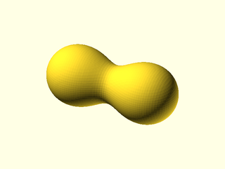
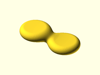
Example 1: Two spheres interacting.
include <BOSL2/std.scad>
include <BOSL2/isosurface.scad>
spec = [
    left(9), mb_sphere(5),
    right(9), mb_sphere(5)
];
metaballs(spec, voxel_size=0.5,
    bounding_box=[[-16,-7,-7], [16,7,7]]);
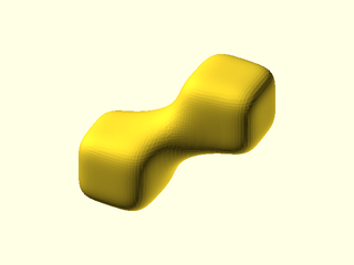
Example 2: Two rounded cuboids interacting.
include <BOSL2/std.scad>
include <BOSL2/isosurface.scad>
spec = [
    move([-8,-5,-5]), mb_cuboid(10),
    move([8,5,5]), mb_cuboid(10)
];
metaballs(spec, voxel_size=0.5,
    bounding_box=[[-15,-12,-12], [15,12,12]]);
Example 3: Two rounded mb_cyl() cones interacting.
include <BOSL2/std.scad>
include <BOSL2/isosurface.scad>
spec = [
    left(10), mb_cyl(15, r1=8, r2=5, rounding=3),
    right(10), mb_cyl(15, r1=8, r2=5, rounding=3)
];
metaballs(spec, voxel_size=0.5,
    bounding_box=[[-19,-9,-10], [19,9,10]]);
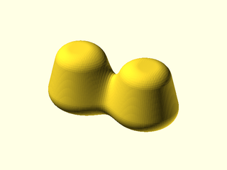
Example 4: Two disks interacting.
include <BOSL2/std.scad>
include <BOSL2/isosurface.scad>
metaballs([
    move([-10,0,2]), mb_disk(5,9),
    move([10,0,-2]), mb_disk(5,9)
    ], 0.5, [[-20,-10,-6], [20,10,6]]);
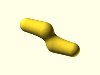
Example 5: Two capsules interacting.
include <BOSL2/std.scad>
include <BOSL2/isosurface.scad>
metaballs([
    move([-8,0,4])*yrot(90), mb_capsule(16,3),
    move([8,0,-4])*yrot(90), mb_capsule(16,3)
    ], 0.5, [[-17,-5,-8], [17,5,8]]);
Example 6: A sphere with two connectors.
include <BOSL2/std.scad>
include <BOSL2/isosurface.scad>
path = [[-20,0,0], [0,0,1], [0,-10,0]];
spec = [
    move(path[0]), mb_sphere(6),
    for(seg=pair(path)) each
       [IDENT, mb_connector(seg[0],seg[1],
        2, influence=0.5)]
];
metaballs(spec, voxel_size=0.5,
    bounding_box=[[-27,-13,-7], [4,7,14]]);
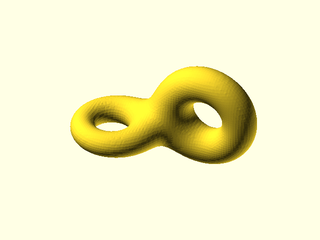
Example 7: Interaction between two tori in different orientations.
include <BOSL2/std.scad>
include <BOSL2/isosurface.scad>
spec = [
    move([-10,0,17]),        mb_torus(r_maj=6, r_min=2),
    move([7,6,21])*xrot(90), mb_torus(r_maj=7, r_min=3)
];
voxelsize = 0.5;
boundingbox = [[-19,-9,9], [18,10,32]];
metaballs(spec, voxelsize, boundingbox);
Example 8: Two octahedrons interacting.
include <BOSL2/std.scad>
include <BOSL2/isosurface.scad>
metaballs([
    move([-10,0,3]), mb_octahedron(8),
    move([10,0,-3]), mb_octahedron(8)
    ], 0.5, [[-21,-11,-13], [21,11,13]]);
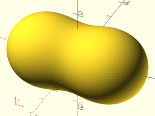
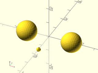
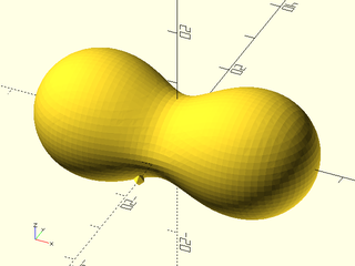
Example 9: These next five examples demonstrate the different types of metaball interactions. We start with two spheres 30 units apart. Each would have a radius of 10 in isolation, but because they are influencing their surroundings, each sphere mutually contributes to the size of the other. The sum of contributions between the spheres add up so that a surface plotted around the region exceeding the threshold defined by isovalue=1 looks like a peanut shape surrounding the two spheres.
include <BOSL2/std.scad>
include <BOSL2/isosurface.scad>
spec = [
    left(15),  mb_sphere(10),
    right(15), mb_sphere(10)
];
voxelsize = 1;
boundingbox = [[-30,-19,-19], [30,19,19]];
metaballs(spec, voxelsize, boundingbox);
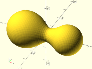
Example 10: Adding a cutoff of 25 to the left sphere causes its influence to disappear completely 25 units away (which is the center of the right sphere). The left sphere is bigger because it still receives the full influence of the right sphere, but the right sphere is smaller because the left sphere has no contribution past 25 units. The right sphere is not abruptly cut off because the cutoff function is smooth and influence is normal. Setting cutoff too small can remove the interactions of one metaball from all other metaballs, leaving that metaball alone by itself.
include <BOSL2/std.scad>
include <BOSL2/isosurface.scad>
spec = [
    left(15),  mb_sphere(10, cutoff=25),
    right(15), mb_sphere(10)
];
voxelsize = 1;
boundingbox = [[-30,-19,-19], [30,19,19]];
metaballs(spec, voxelsize, boundingbox);
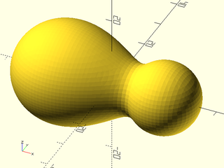
Example 11: Here, the left sphere has less influence in addition to a cutoff. Setting influence=0.5 results in a steeper falloff of contribution from the left sphere. Each sphere has a different size and shape due to unequal contributions based on distance.
include <BOSL2/std.scad>
include <BOSL2/isosurface.scad>
spec = [
    left(15),  mb_sphere(10, influence=0.5, cutoff=25),
    right(15), mb_sphere(10)
];
voxelsize = 1;
boundingbox = [[-30,-19,-19], [30,19,19]];
metaballs(spec, voxelsize, boundingbox);
Example 12: In this example, we have two size-10 spheres as before and one tiny sphere of 1.5 units radius offset a bit on the y axis. With an isovalue of 1, this figure would appear similar to Example 9 above, but here the isovalue has been set to 2, causing the surface to shrink around a smaller volume values greater than 2. Remember, higher isovalue thresholds cause metaballs to shrink.
include <BOSL2/std.scad>
include <BOSL2/isosurface.scad>
spec = [
   left(15),  mb_sphere(10),
   right(15), mb_sphere(10),
   fwd(15),   mb_sphere(1.5)
];
voxelsize = 1;
boundingbox = [[-30,-19,-19], [30,19,19]];
metaballs(spec, voxelsize, boundingbox,
    isovalue=2);
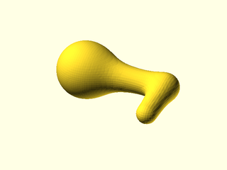
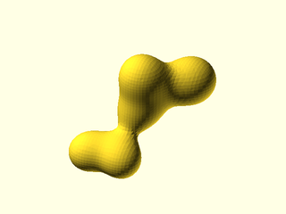
Example 13: Keeping isovalue=2, the influence of the tiny sphere has been set quite high, to 10. Notice that the tiny sphere shrinks a bit, but it has dramatically increased its contribution to its surroundings, causing the two other spheres to grow and meld into each other. The influence argument on a small metaball affects its surroundings more than itself.
include <BOSL2/std.scad>
include <BOSL2/isosurface.scad>
spec = [
   move([-15,0,0]), mb_sphere(10),
   move([15,0,0]),  mb_sphere(10),
   move([0,-15,0]), mb_sphere(1.5, influence=10)
];
voxelsize = 1;
boundingbox = [[-30,-19,-19], [30,19,19]];
metaballs(spec, voxelsize, boundingbox,
    isovalue=2);
Example 14: A group of five spherical metaballs with different sizes. The parameter show_stats=true (not shown here) was used to find a compact bounding box for this figure.
include <BOSL2/std.scad>
include <BOSL2/isosurface.scad>
spec = [ // spheres of different sizes
    move([-20,-20,-20]), mb_sphere(5),
    move([0,-20,-20]),   mb_sphere(4),
    IDENT,               mb_sphere(3),
    move([0,0,20]),      mb_sphere(5),
    move([20,20,10]),    mb_sphere(7)
];
voxelsize = 1.5;
boundingbox = [[-30,-31,-31], [32,31,31]];
metaballs(spec, voxelsize, boundingbox);
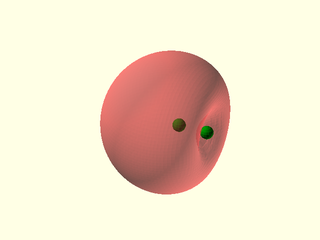
Example 15: A metaball can be negative. In this case we have two metaballs in close proximity, with the small negative metaball creating a dent in the large positive one. The positive metaball is shown transparent, and small spheres show the center of each metaball. The negative metaball isn't visible because its field is negative; the isosurface encloses only field values greater than the isovalue of 1.
include <BOSL2/std.scad>
include <BOSL2/isosurface.scad>
centers = [[-1,0,0], [1.25,0,0]];
spec = [
    move(centers[0]), mb_sphere(8),
    move(centers[1]), mb_sphere(3, negative=true)
];
voxelsize = 0.25;
isovalue = 1;
boundingbox = [[-7,-6,-6], [3,6,6]];
#metaballs(spec, voxelsize, boundingbox, isovalue);
color("green") move_copies(centers) sphere(d=1, $fn=16);
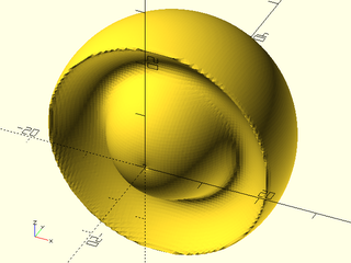
Example 16: When a positive and negative metaball interact, the negative metaball reduces the influence of the positive one, causing it to shrink, but not disappear because its contribution approaches infinity at its center. In this example we have a large positive metaball near a small negative metaball at the origin. The negative ball as high influence, and a cutoff limiting its influence to 20 units. The negative metaball influences the positive one up to the cutoff, causing the positive metaball to appear smaller inside the cutoff range, and appear its normal size outside the cutoff range. The positive metaball has a small dimple at the origin (the center of the negative metaball) because it cannot overcome the infinite negative contribution of the negative metaball at the origin.
include <BOSL2/std.scad>
include <BOSL2/isosurface.scad>
spec = [
    back(10), mb_sphere(20),
    IDENT, mb_sphere(2, influence=30,
                     cutoff=20, negative=true),
];
voxelsize = 0.5;
boundingbox = [[-20,-4,-20], [20,30,20]];
metaballs(spec, voxelsize, boundingbox);
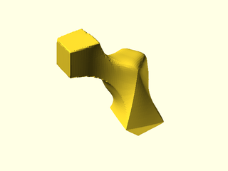
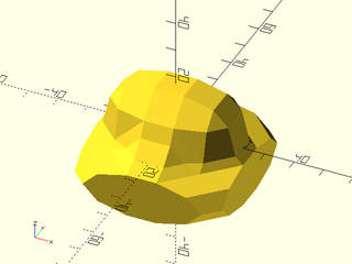
Example 17: A cube, a rounded cube, and an octahedron interacting. Because the surface is generated through cubical voxels, voxel corners are always cut off, resulting in difficulty resolving some sharp edges.
include <BOSL2/std.scad>
include <BOSL2/isosurface.scad>
spec = [
    move([-7,-3,27])*zrot(55), mb_cuboid(6, squareness=1),
    move([5,5,21]),   mb_cuboid(5),
    move([10,0,10]),  mb_octahedron(5)
];
voxelsize = 0.5; // a bit slow at this resolution
boundingbox = [[-12,-9,3], [18,10,32]];
metaballs(spec, voxelsize, boundingbox);
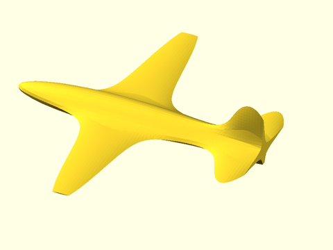
Example 18: A toy airplane, constructed only from metaball spheres with scaling. The bounding box is used to clip the wingtips, tail, and belly of the fuselage.
include <BOSL2/std.scad>
include <BOSL2/isosurface.scad>
bounding_box = [[-55,-50,-5],[35,50,17]];
spec = [
    move([-20,0,0])*scale([25,4,4]),   mb_sphere(1), // fuselage
    move([30,0,5])*scale([4,0.5,8]),   mb_sphere(1), // vertical stabilizer
    move([30,0,0])*scale([4,15,0.5]),  mb_sphere(1), // horizontal stabilizer
    move([-15,0,0])*scale([6,45,0.5]), mb_sphere(1)  // wing
];
voxel_size = 1;
metaballs(spec, voxel_size, bounding_box);
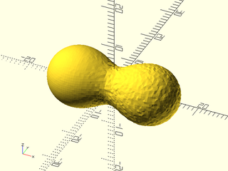
Example 19: Demonstration of a custom metaball function, in this case a sphere with some random noise added to its value. The dv argument must be first; it is calculated internally as a distance vector from the metaball center to a probe point inside the bounding box, and you convert it to a scalar distance dist that is calculated inside your function (dist could be a more complicated expression, depending on the shape of the metaball). The call to mb_cutoff() at the end handles the cutoff function for the noisy ball consistent with the other internal metaball functions; it requires dist and cutoff as arguments. You are not required to include the cutoff and influence arguments in a custom function, but this example shows how.
include <BOSL2/std.scad>
include <BOSL2/isosurface.scad>
function noisy_sphere(dv, r, noise_level, cutoff=INF, influence=1) =
    let(
        noise = rands(0, noise_level, 1)[0],
        dist = norm(dv) + noise
    ) mb_cutoff(dist,cutoff) * (r/dist)^(1/influence);

spec = [
    left(9),  mb_sphere(5),
    right(9), function (dv) noisy_sphere(dv, 5, 0.2),
];
voxelsize = 0.5;
boundingbox = [[-16,-8,-8], [16,8,8]];
metaballs(spec, voxelsize, boundingbox);
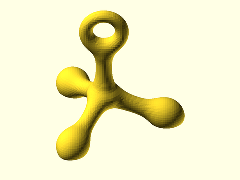
Example 20: A complex example using ellipsoids, a capsule, spheres, and a torus to make a tetrahedral object with rounded feet and a ring on top. The bottoms of the feet are flattened by clipping with the bottom of the bounding box. The center of the object is thick due to the contributions of three ellipsoids and a capsule converging. Designing an object like this using metaballs requires trial and error with low-resolution renders.
include <BOSL2/std.scad>
include <BOSL2/isosurface.scad>
include <BOSL2/polyhedra.scad>
tetpts = zrot(15, p = 22 * regular_polyhedron_info("vertices", "tetrahedron"));
tettransform = [ for(pt = tetpts) move(pt)*rot(from=RIGHT, to=pt)*scale([7,1.5,1.5]) ];

spec = [
    // vertical cylinder arm
    up(15), mb_capsule(17, 2, influence=0.8),
    // ellipsoid arms
    for(i=[0:2]) each [tettransform[i], mb_sphere(1, cutoff=30)],
    // ring on top
    up(35)*xrot(90), mb_torus(r_maj=8, r_min=2.5, cutoff=35),
    // feet
    for(i=[0:2]) each [move(2.2*tetpts[i]), mb_sphere(5, cutoff=30)],
];
voxelsize = 1;
boundingbox = [[-22,-32,-13], [36,32,46]];
// useful to save as VNF for copies and manipulations
vnf = metaballs(spec, voxelsize, boundingbox, isovalue=1);
vnf_polyhedron(vnf);
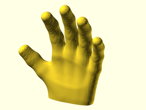
Example 21: This example demonstrates grouping metaballs together and nesting them in lists of other metaballs, to make a crude model of a hand. Here, just one finger is defined, and a thumb is defined from one less joint in the finger. Individual fingers are grouped together with different positions and scaling, along with the thumb. Finally, this group of all fingers is used to combine with a rounded cuboid, with a slight ellipsoid dent subtracted to hollow out the palm, to make the hand.
include <BOSL2/std.scad>
include <BOSL2/isosurface.scad>
joints = [[0,0,1], [0,0,85], [0,-5,125], [0,-16,157], [0,-30,178]];
finger = [
    for(i=[0:3]) each
        [IDENT, mb_connector(joints[i], joints[i+1], 9+i/5, influence=0.22)]
];
thumb = [
    for(i=[0:2]) each [
        scale([1,1,1.2]),
        mb_connector(joints[i], joints[i+1], 9+i/2, influence=.28)
    ]
];
allfingers = [
    left(15)*zrot(5)*yrot(-50)*scale([1,1,0.6])*zrot(30), thumb,
    left(15)*yrot(-9)*scale([1,1,0.9]), finger,
    IDENT, finger,
    right(15)*yrot(8)*scale([1,1,0.92]), finger,
    right(30)*yrot(17)*scale([0.9,0.9,0.75]), finger
];
hand = [
    IDENT, allfingers,
    move([-5,0,5])*scale([1,0.36,1.55]), mb_cuboid(90, squareness=0.3, cutoff=80),
    move([-10,-95,50])*yrot(10)*scale([2,2,0.95]),
        mb_sphere(r=15, cutoff=50, influence=1.5, negative=true)
];
voxsize=2.5;
bbox = [[-104,-40,-10], [79,18,188]];
metaballs(hand, voxsize, bbox, isovalue=1);
Function/Module: isosurface()
Synopsis: Creates a 3D isosurface (a 3D contour) from a function or array of values. [Geom] [VNF]
Topics: Isosurfaces, VNF Generators
Usage: As a module
- isosurface(f, isovalue, voxel_size, bounding_box, [reverse=], [closed=], [show_stats=], ...) [ATTACHMENTS];
Usage: As a function
- vnf = isosurface(f, isovalue, voxel_size, bounding_box, [reverse=], [closed=], [show_stats=]);
Description:
Computes a VNF structure of a 3D isosurface within a bounded box at a single
isovalue or range of isovalues.
The isosurface of a function f(x,y,z) is the set of points where f(x,y,z)=c for some
constant isovalue, c.
To provide a function you supply a function literal
taking three parameters as input to define the grid coordinate location (e.g. x,y,z) and
returning a single numerical value.
You can also define an isosurface using a 3D array of values instead of a function, in which
case the isosurface is the set of points equal to the isovalue as interpolated from the array.
The array indices are in the order [x][y][z].
The VNF that is computed has the isosurface as its bounding surface, with all the points where
f(x,y,z)>c on the interior side of the surface.
When the isovalue is a range, [c1, c2], then the resulting VNF has two bounding surfaces
corresponding to c1 and c2, and the interior of the object are the points with intermediate
isovalues; this generally produces a shell object that has an inside and outside surface. The
range can start at -INF or end at INF. A single isovalue c is equivalent to [c,INF].
The isosurface is evaluated over a bounding box defined by its minimum and maximum corners,
[[xmin,ymin,zmin],[xmax,ymax,zmax]]. This bounding box is divided into voxels of the
specified voxel_size. Smaller voxels produce a finer, smoother result at the expense of
execution time. If the voxel size doesn't exactly divide your specified bounding box, then
the bounding box is enlarged to contain whole voxels, and centered on your requested box. If
the bounding box clips the isosurface and closed=true (the default), a surface is added to create
a closed manifold object. Setting closed=false causes the VNF to end at the bounding box,
resulting in a non-manifold shape that exposes the inside of the object.
The voxel_size and bounding_box parameters affect the run time, which can be long.
A voxel size of 1 with a bounding box volume of 200×200×200 may be slow because it requires the
calculation and storage of 8,000,000 function values, and more processing and memory to generate
the triangulated mesh. On the other hand, a voxel size of 5 over a 100×100×100 bounding box
requires only 8,000 function values and a modest computation time. A good rule is to keep the
number of voxels below 10,000 for preview, and adjust the voxel size smaller for final
rendering. A bounding box that is larger than your isosurface wastes time computing function
values that are not needed. If the isosurface fits completely within the bounding box, you can
call pointlist_bounds() on vnf[0] returned from the isosurface() function to get an
idea of a the optimal bounding box to use. You may be able to decrease run time, or keep the
same run time but increase the resolution. You can also set the parameter show_stats=true to
get the bounds of the voxels containing the surface.
The point list in the VNF structure contains many duplicated points. This is not a
problem for rendering the shape, but if you want to eliminate these, you can pass
the structure to vnf_merge_points(). Additionally, flat surfaces (often
resulting from clipping by the bounding box) are triangulated at the voxel size
resolution, and these can be unified into a single face by passing the vnf
structure to vnf_unify_faces(). These steps can be computationally expensive
and are not normally necessary.
Arguments:
| By Position | What it does |
|---|---|
f |
The isosurface function or array. |
isovalue |
a scalar giving the isovalue parameter or a 2-vector giving an isovalue range. |
voxel_size |
scalar size of the voxel cube that is used to sample the surface. |
bounding_box |
When f is a function, a pair of 3D points [[xmin,ymin,zmin], [xmax,ymax,zmax]], specifying the minimum and maximum corner coordinates of the bounding box. The actual bounding box enlarged if necessary to make the voxels fit perfectly, and centered around your requested box. When f is an array of values, bounding_box is already implied by the array size combined with voxel_size, in which case this implied bounding box is centered around the origin. |
| By Name | What it does |
|---|---|
closed |
When true, close the surface if it intersects the bounding box by adding a closing face. When false, do not add a closing face and instead produce a non-manfold VNF that has holes. Default: true |
reverse |
When true, reverses the orientation of the VNF faces. Default: false |
show_stats |
If true, display statistics in the console window about the isosurface: number of voxels that contain the surface, number of triangles, bounding box of the voxels, and voxel-rounded bounding box of the surface, which may help you reduce your bounding box to improve speed. Enabling this parameter has a slight speed penalty. Default: false |
convexity |
Maximum number of times a line could intersect a wall of the shape. Affects preview only. Default: 6 |
cp |
(Module only) Center point for determining intersection anchors or centering the shape. Determines the base of the anchor vector. Can be "centroid", "mean", "box" or a 3D point. Default: "centroid" |
anchor |
(Module only) Translate so anchor point is at origin (0,0,0). See anchor. Default: "origin" |
spin |
(Module only) Rotate this many degrees around the Z axis after anchor. See spin. Default: 0 |
orient |
(Module only) Vector to rotate top toward, after spin. See orient. Default: UP |
atype |
(Module only) Select "hull" or "intersect" anchor type. Default: "hull" |
Anchor Types:
| Anchor Type | What it is |
|---|---|
| "hull" | Anchors to the virtual convex hull of the shape. |
| "intersect" | Anchors to the surface of the shape. |
Named Anchors:
| Anchor Name | Position |
|---|---|
| "origin" | Anchor at the origin, oriented UP. |
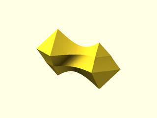
Example 1: A gyroid is an isosurface defined by all the zero values of a 3D periodic function. To illustrate what the surface looks like, closed=false has been set to expose both sides of the surface. The surface is periodic and tileable along all three axis directions. This a non-manifold surface as displayed, not useful for 3D modeling. This example also demonstrates using an additional parameter in the field function beyond just x,y,z; in this case controls the wavelength of the gyroid.
include <BOSL2/std.scad>
include <BOSL2/isosurface.scad>
function gyroid(x,y,z, wavelength) = let(
    p = 360/wavelength,
    px = p*x, py = p*y, pz = p*z
) sin(px)*cos(py) + sin(py)*cos(pz) + sin(pz)*cos(px);
isovalue = 0;
bbox = [[-100,-100,-100], [100,100,100]];
isosurface(function (x,y,z) gyroid(x,y,z, wavelength=200),
    isovalue, voxel_size=5, bounding_box=bbox,
    closed=false);
Example 2: If we remove the closed parameter or set it to true, the isosurface algorithm encloses the entire half-space bounded by the "inner" gyroid surface, leaving only the "outer" surface exposed. This is a manifold shape but not what we want if trying to model a gyroid.
include <BOSL2/std.scad>
include <BOSL2/isosurface.scad>
function gyroid(x,y,z, wavelength) = let(
    p = 360/wavelength,
    px = p*x, py = p*y, pz = p*z
) sin(px)*cos(py) + sin(py)*cos(pz) + sin(pz)*cos(px);
isovalue = 0;
bbox = [[-100,-100,-100], [100,100,100]];
isosurface(function (x,y,z) gyroid(x,y,z, wavelength=200),
    isovalue, voxel_size=5, bounding_box=bbox);
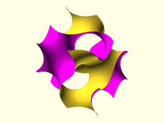
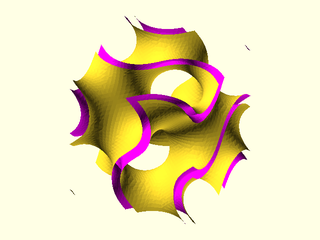
Example 3: To make the gyroid a double-sided surface, we need to specify a small range around zero for isovalue. Now we have a double-sided surface although with closed=false the edges are not closed where the surface is clipped by the bounding box.
include <BOSL2/std.scad>
include <BOSL2/isosurface.scad>
function gyroid(x,y,z, wavelength) = let(
    p = 360/wavelength,
    px = p*x, py = p*y, pz = p*z
) sin(px)*cos(py) + sin(py)*cos(pz) + sin(pz)*cos(px);
isovalue = [-0.3, 0.3];
bbox = [[-100,-100,-100], [100,100,100]];
isosurface(function (x,y,z) gyroid(x,y,z, wavelength=200),
    isovalue, voxel_size=5, bounding_box=bbox,
    closed = false);
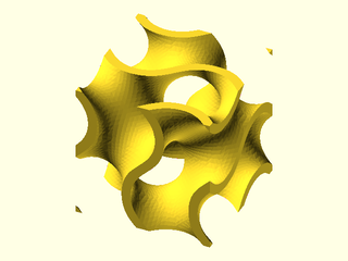
Example 4: To make the gyroid a valid manifold 3D object, we remove the closed parameter (same as setting closed=true), which closes the edges where the surface is clipped by the bounding box. The resulting object can be tiled, the VNF returned by the functional version can be wrapped around an axis using vnf_bend(), and other operations.
include <BOSL2/std.scad>
include <BOSL2/isosurface.scad>
function gyroid(x,y,z, wavelength) = let(
    p = 360/wavelength,
    px = p*x, py = p*y, pz = p*z
) sin(px)*cos(py) + sin(py)*cos(pz) + sin(pz)*cos(px);
isovalue = [-0.3, 0.3];
bbox = [[-100,-100,-100], [100,100,100]];
isosurface(function (x,y,z) gyroid(x,y,z, wavelength=200),
    isovalue, voxel_size=5, bounding_box=bbox);
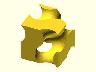
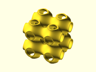
Example 5: An approximation of the triply-periodic minimal surface known as Schwartz P.
include <BOSL2/std.scad>
include <BOSL2/isosurface.scad>
function schwartz_p(x,y,z, wavelength) = let(
    p = 360/wavelength,
    px = p*x, py = p*y, pz = p*z
)  cos(px) + cos(py) + cos(pz);
isovalue = [-0.2, 0.2];
bbox = [[-100,-100,-100], [100,100,100]];
isosurface(function (x,y,z) schwartz_p(x,y,z, 100),
    isovalue, voxel_size=4, bounding_box=bbox);
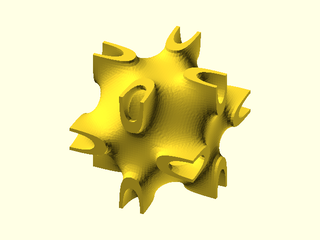
Example 6: Another approximation of the triply-periodic minimal surface known as Neovius.
include <BOSL2/std.scad>
include <BOSL2/isosurface.scad>
function neovius(x,y,z, wavelength) = let(
    p = 360/wavelength,
    px = p*x, py = p*y, pz = p*z
)  3*(cos(px) + cos(py) + cos(pz)) + 4*cos(px)*cos(py)*cos(pz);
 isovalue = [-0.3, 0.3];
bbox = [[-100,-100,-100], [100,100,100]];
isosurface(function (x,y,z) neovius(x,y,z,200),
    isovalue, voxel_size=4, bounding_box=bbox);
Example 7: Using an array for the f argument instead of a function literal.
include <BOSL2/std.scad>
include <BOSL2/isosurface.scad>
field = [
  repeat(0,[6,6]),
  [ [0,1,2,2,1,0],
    [1,2,3,3,2,1],
    [2,3,4,4,3,2],
    [2,3,4,4,3,2],
    [1,2,3,3,2,1],
    [0,1,2,2,1,0]
  ],
  [ [0,0,0,0,0,0],
    [0,0,1,1,0,0],
    [0,2,3,3,2,0],
    [0,2,3,3,2,0],
    [0,0,1,1,0,0],
    [0,0,0,0,0,0]
  ],
  [ [0,0,0,0,0,0],
    [0,0,0,0,0,0],
    [0,1,2,2,1,0],
    [0,1,2,2,1,0],
    [0,0,0,0,0,0],
    [0,0,0,0,0,0]
  ],
  repeat(0,[6,6])
];
rotate([0,-90,180])
   isosurface(field, isovalue=0.5,
       voxel_size=10);